System Design from First Principles: Reconstructing the Digital Universe
The systems we build are conversations between physics and information: latency is just distance; throughput is just concurrency; reliability is controlled entropy. You don’t “add a cache” so much as reshape probability distributions; you don’t “scale a service” so much as manage queueing regimes. When the abstractions leak, the physics shows through—and that’s where real design begins.
This guide is the result of re-deriving the stack from first principles. For every layer, we’ll pin down the why (constraints from information theory and distributed consensus), the how (algorithms, data structures, deployment patterns), and the what (code, equations, and runbooks). Each chapter opens with a Mermaid chart to anchor the mental model before we dive deep.
The Genesis: System Design From Physics point of view
System design is not about technology; it is about the physics of information flow. Every distributed system is an organism made of four primitives:
- Scalability: cost and complexity grow sub-linearly with load.
- Maintainability: simple contracts, clear ownership, low cognitive load.
- Efficiency: maximize work per joule/$ and minimize wasted motion (unnecessary hops, copies, waits).
- Resilience: failure is expected; blast radius is limited; recovery is automatic.
A good design plans for failure as a first-class behavior, not an afterthought.
First principles.
- Little’s Law: (L=\lambda W). If arrival rate (\lambda) is fixed, any increase in latency (W) linearly inflates in-flight work (L). That’s how cascading failures begin.
- Utilization law: with service rate (\mu), utilization (\rho=\lambda/\mu). For M/M/1, (W=\frac{1}{\mu-\lambda}): as (\rho \to 1), latency explodes. Hence autoscaling and load shedding are not luxuries; they’re stability conditions.
- Tail at scale: If a request fans out to (n) backends, p99 of each becomes worse than p99 of the end-to-end. Use hedged requests, partial results, or quorum reads.
Error budgets and release velocity. Given SLO (a), error budget (b=1-a). Control loop: increase rollout rate until measured burn rate > threshold; then pause rollouts. This is a PID controller on reliability.
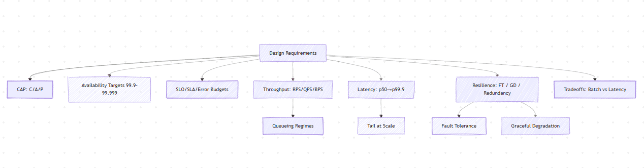
Batch vs latency. Batch maximizes throughput (lower per-item overhead) but increases (W). Streaming minimizes (W) but increases coordination overhead. Choose based on cost of staleness and value of freshness.
CAP and the Geometry of Trade-offs
Distributed systems live in a geometry constrained by Consistency (C), Availability (A), and Partition tolerance (P). But CAP is not a choice — it is a projection of physical laws: no information can propagate faster than the network latency between nodes.
Let ( t_p ) be partition duration, and ( t_c ) the time needed to achieve consensus. If ( t_p > t_c ), the system can be consistent and available. If ( t_p \approx t_c ), you must choose.
Mathematically, the CAP theorem is a corollary of the FLP impossibility in asynchronous systems. The FLP result states:
In an asynchronous distributed system, it is impossible to guarantee both safety (consistency) and liveness (availability) in the presence of even one faulty process.
Most real systems move dynamically within it:
- ZooKeeper favors CP.
- DynamoDB favors AP.
- Spanner approximates CA using synchronized clocks (TrueTime).
Design rule: make inconsistency explicit (timestamps, versions, CRDTs, read-repair) when choosing AP.
Availability, reliability, redundancy
Uptime math (per year):
| Availability | Max downtime/year |
|---|---|
| 99.9% | ~8.76 hours |
| 99.99% | ~52.6 minutes |
| 99.999% | ~5.26 minutes |
To reach a target, compose layers: overall availability ≈ product of stage availabilities. Avoid a strong link backed by weak dependencies.
Mechanics:
- Redundancy: N+1, multi-AZ/region, diverse providers where warranted.
- Fault tolerance: quorum writes, retry with jitter, backpressure, circuit breakers.
- Graceful degradation: serve cached/partial results, disable noncritical features, lower fidelity.
SLOs and SLAs (contracts)
- SLO (internal): measurable target that guides engineering (e.g., p99 latency < 300 ms, 99.95% availability/month).
- SLA (external): customer-facing commitment (credits/penalties if breached).
- Error budget: (1-\text{SLO}). Spend it (deploy faster) until burn rate triggers a freeze.
Good SLOs are few, tied to user-visible outcomes, and cheap to measure (RED/USE dashboards).
Throughput & latency (the physics)
- Throughput: work per unit time — RPS/QPS/BPS.
- Latency: time per request. Track distributions, not averages (p50, p95, p99, p99.9).
Queueing laws (back-of-envelope):
- Little’s Law: (L = \lambda W) (in-flight = arrival rate × latency).
- M/M/1 waiting time: (W \approx \frac{1}{\mu-\lambda}). As utilization ( \rho=\lambda/\mu \to 1), latency explodes.
- Fan-out tail: with (n) parallel calls, end-to-end tail ≫ per-call tail. Use hedging, timeouts, fallbacks, or partial quorums.
Typical trade-offs:
- Batching ↑throughput, ↑latency.
- Replication ↑availability, ↑consistency cost (coordination).
- Caching ↓latency, may serve stale data (tune TTL/ETag/validation).
Computer Architecture — When Information Meets Physics
Let us start from bits and bytes, the atoms of information. Claude Shannon’s entropy equation tells us the theoretical limit of information in a signal:
[ H(X) = -\sum_i p(x_i)\log_2 p(x_i) ]
Every data structure and storage medium is a way of preserving or transforming entropy.
Memory Hierarchy as a Thermodynamic Gradient
| Layer | Typical Latency | Example | Analogy |
|---|---|---|---|
| L1 cache | ~1 ns | CPU register cache | Kinetic energy |
| L2 cache | ~3–10 ns | Private core cache | Local thermal zone |
| L3 cache | ~30–50 ns | Shared CPU cache | Shared heat reservoir |
| DRAM | ~100 ns | Main memory | Thermal diffusion |
| SSD | ~100 µs | NVMe | Potential energy barrier |
| HDD | ~10 ms | Rotational disk | Cold storage, entropy sink |
Latency increases exponentially as we descend the memory pyramid. Hence, a single cache miss propagates as a wave of entropy. Efficient systems minimize cross-layer transitions — locality is not an optimization, it’s a law of energy efficiency.
As size exceeds cache boundaries, the access time per element jumps — a live demonstration of the cache boundary effect.
Caching as an Information-Theoretic Problem
A cache is an entropy compressor. It increases predictability by reusing the most probable requests.
Let ( p_i ) be the probability of accessing item ( i ), and ( C ) the cache size. The expected hit rate under Least-Recently-Used (LRU) can be approximated as:
[ H(C) = \frac{\sum_{i=1}^{C} p_i}{\sum_{i=1}^{N} p_i} ]
This shows why Zipf’s Law (popularity ∝ 1/rank) makes caching effective: a small subset of data covers a large fraction of requests.
Code: Simulating Cache Hit Ratio
import numpy as np

def zipf_cache_hit(alpha=1.2, n_items=10000, cache_size=100):
    ranks = np.arange(1, n_items+1)
    probs = 1 / np.power(ranks, alpha)
    probs /= np.sum(probs)
    return np.sum(probs[:cache_size])

for c in [10, 100, 1000, 5000]:
    print(f"Cache {c}: hit ratio {zipf_cache_hit(cache_size=c):.3f}")
The resulting curve is logarithmic — diminishing returns after the “head” of the distribution is cached.
Networking — Time, Causality, and Entropy Flow
Network design is the physics of distributed causality. Every packet carries both data and uncertainty.
TCP Handshake
Each TCP connection requires:
- SYN
- SYN-ACK
- ACK
That’s three round-trip times (RTTs) before data flow begins. At 100 ms RTT (inter-continental), this alone adds 300 ms latency. Thus QUIC/HTTP3 moves to UDP to eliminate head-of-line blocking and handshake costs.
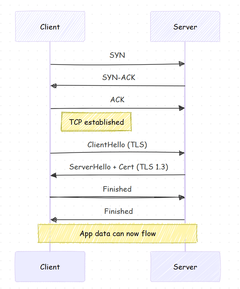
TCP costs. Three-way handshake = 1–1.5 RTTs before payload. With TLS 1.2, add another RTT; TLS 1.3/QUIC reduces it. In cross-region paths (100–180ms RTT), handshake dominates.
Congestion control. Reno/CUBIC/BBR pick different equilibria between throughput and latency. BBR targets bandwidth-delay product, often reducing bufferbloat tails.
DNS as a Global Consensus Layer
DNS resolution introduces its own distributed consistency problem. The hierarchy (root → TLD → authoritative) is essentially a read-optimized DHT with caching TTLs balancing freshness vs load.
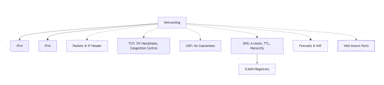
IP addressing
- IPv4: 32-bit (~4.3B addresses). CIDR (e.g., 10.0.0.0/8).
- IPv6: 128-bit, addresses exhaustion solved; mandatory IPsec; different header layout.
- Public vs Private: RFC1918 ranges (10/8, 172.16/12, 192.168/16). NAT maps private↔public.
- Static vs Dynamic: servers prefer static; clients often DHCP.
IP headers (essential fields)
- v4: Version, IHL, DSCP/ECN, Total Length, Identification, Flags/Fragment Offset, TTL, Protocol (6=TCP,17=UDP), Header Checksum, Src/Dst IP.
- v6: Version, Traffic Class, Flow Label, Payload Length, Next Header, Hop Limit, Src/Dst IP.
TCP vs UDP
- TCP: connection-oriented, reliable, ordered, congestion-controlled. Handshake (SYN→SYN/ACK→ACK), byte stream, retransmission, flow control (rwnd), congestion control (CUBIC/BBR).
- UDP: connectionless, best-effort, unordered; low overhead; used for RTP/VoIP, QUIC, DNS. App must add reliability if needed.
DNS (name→address)
- Resolver path: stub → recursive → (root → TLD → authoritative).
- Records: A(IPv4), AAAA(IPv6), CNAME, NS, MX, TXT, SRV). TTL = freshness vs load.
- ICANN/registrars govern namespace; anycast improves RTT & resilience.
Production notes
- Tune TCP keepalive, initial congestion window, and MSS/MTU to avoid fragmentation.
- Prefer HTTP/3 (QUIC over UDP) for long-haul/high loss links.
- Set sane DNS TTLs (e.g., 60–300s) for fast failover; longer for static assets.
Application Layer Protocols
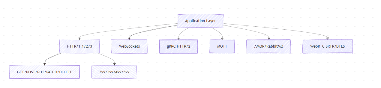
HTTP
- Request-response, stateless; semantics live in method + path + headers + body.
- /2: multiplexed streams over one TCP; /3: QUIC removes TCP head-of-line.
- Cache controls:
Cache-Control,ETag,Last-Modified,Vary.
WebSockets
- Full-duplex channel upgraded from HTTP. Great for chat, tickers, collaborative editing. Requires heartbeat/ping-pong, backpressure.
WebRTC
- Browser-to-browser audio/video/data; STUN/TURN/ICE to traverse NAT; SRTP for media; tight latency budgets.
MQTT
- Lightweight pub/sub, QoS 0/1/2; ideal for IoT (low bandwidth, intermittent links).
AMQP
- Enterprise messaging (queues, exchanges, routing keys, acks, dead-letter). Good for exactly-once-ish workflows with idempotent sinks.
RPC (gRPC)
- Strongly typed contracts (Protobuf), bidi streams, deadlines/cancellation. Choose for service-to-service low-latency calls.
Production notes
- Prefer gRPC for internal microservices; HTTP/REST for public APIs.
- Add deadlines/timeouts, idempotency, and cancellation to all RPCs.
- For real-time UIs: prefer WebSockets or Server-Sent Events; use WebRTC for A/V.
API Design — The Interface of Systems
Paradigms
- REST: simple resources, cacheable, great for browsers; risk of over/under-fetching.
- GraphQL: client-driven selection; fewer roundtrips; needs depth limits, cost analysis.
- gRPC: Protobuf contracts; fastest on service mesh; not browser-native.
CRUD skeleton (REST)
POST /products(create)GET /products?limit&cursor&filter=...(list with cursor pagination, not offset)GET /products/{id}(read)PATCH /products/{id}(partial update)DELETE /products/{id}(delete)
Idempotency
- Non-safe methods use
Idempotency-Key. Server stores key→result for TTL to dedupe retries.
Versioning
- URL (/v1/...) for breaking changes;
- Additive evolution (optional fields) to avoid frequent major bumps (esp. GraphQL).
Rate limiting & quotas
- Token bucket/Leaky bucket per user/apiKey/ip. Return 429 with Retry-After.
CORS (browser)
- Tight allowlist; preflight caching; minimal exposed headers.
Production notes
- Document with OpenAPI/Protobuf; generate SDKs.
- Enforce timeouts, resource limits, and SLIs (Rate/Errors/Duration) per route.
- Add request IDs and propagate traceparent.
Caching and CDNs
Where to cache
- Browser: static assets; governed by Cache-Control, ETag.
- CDN edge: global latency reduction, TLS offload, DDoS mitigation.
- Server/in-memory (Redis/Memcached): hot keys, session/state, precomputed views.
- DB cache/result cache: avoid repeated expensive queries.
Write policies
- Write-around: write to DB only; cache on read-miss (simpler writes, more read misses).
- Write-through: write to DB and cache (consistent cache, slower writes).
- Write-back: write to cache, flush later (fast writes, durability risk → require WAL/replication).
Eviction
- LRU/LFU/FIFO; beware stampedes → use request coalescing and TTL jitter.
CDNs
- Pull: edge fetches from origin on first request (lower ops overhead).
- Push: you upload to CDN storage (great for large, rarely changing artifacts).
- Use immutable asset versioning (/app.css?v=hash) + long TTLs.
Measuring effectiveness
- Hit ratio, origin offload, p95/99 latency, error rate at edge vs origin.
Production notes
- Invalidate precisely (path, tag, surrogate keys) to avoid “nuke the edge.”
- For dynamic HTML, combine edge caching with stale-while-revalidate or edge compute.
- Protect DB with read-through caches, but keep authoritative writes consistent (idempotent mutations, transactions).
Databases — The Thermodynamics of State
A database is a system that resists entropy growth in persistent state.
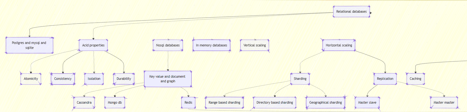
ACID and the Arrow of Time
- Atomicity: No partial state.
- Consistency: State transitions obey invariants.
- Isolation: Concurrent transactions appear serial.
- Durability: State survives crash — information persists beyond entropy spikes.
Durability converts transient electric charges into magnetic or solid-state configurations — a literal battle against the second law of thermodynamics.
Scaling Laws
Horizontal scalability through sharding redistributes entropy spatially: [ T_{global} = \sum_i T_{shard} + T_{coord} ] where ( T_{coord} ) is coordination overhead. Minimizing ( T_{coord} ) is the core of scalable design — why eventual consistency wins at scale.
Replication and Causal Order
Causal consistency ensures that if event A → B, then every replica sees A before B. Vector clocks approximate this causal order with ( O(n) ) space complexity — a trade-off between accuracy and cost.
Data Engineering — Orchestrating the Flow of Reality
From Ingestion to Transformation
Modern pipelines are cybernetic systems: sensors (CDC), actuators (ETL jobs), and feedback loops (data quality metrics).

Each edge introduces latency, each node introduces entropy. The art is minimizing both while preserving lineage.
The DAG as a Knowledge Graph
Airflow’s DAG is not merely a schedule; it’s a computational graph akin to a neural net. Each node’s output becomes another’s input, representing information conservation. Hence, idempotency and replayability are essential: they ensure temporal determinism in asynchronous systems.
Machine Learning Engineering — Turning Entropy into Prediction
Machine learning extends system design from deterministic computation to probabilistic computation.
Feature Store as an Information Reservoir
Features represent compressed domain knowledge. The offline store (batch) and online store (real-time) are two views of the same underlying distribution ( P(X, Y) ).
Maintaining statistical consistency between them is a synchronization problem, akin to maintaining cache coherence between memory levels.
The ML Lifecycle as a Closed Loop
Data → Feature Extraction → Model Training → Evaluation → Deployment → Monitoring → Data
Each arrow closes the cybernetic feedback loop — learning occurs when monitoring re-informs data selection.
Drift Detection
Let baseline distribution be ( P_0(X) ) and current ( P_t(X) ). We detect drift when [ D_{KL}(P_t || P_0) > \epsilon ] where ( D_{KL} ) is Kullback-Leibler divergence. A practical monitoring system approximates this via streaming histograms.
import numpy as np
def kl_div(p, q):
    p, q = np.asarray(p), np.asarray(q)
    return np.sum(np.where(p != 0, p * np.log(p / q), 0))
When divergence exceeds threshold, retraining is triggered — an autonomous learning reflex.
Operations and Reliability — Cybernetic Control of Chaos
Observability as Information Feedback
Observability transforms logs, metrics, and traces into state estimation. If we model a service as a dynamical system:
[ x_{t+1} = f(x_t, u_t) + \eta_t ] [ y_t = h(x_t) + \epsilon_t ]
then logging provides ( y_t ) (outputs), and SRE practices estimate hidden state ( x_t ). Prometheus and Grafana are not dashboards — they are real-time observers minimizing uncertainty ( H(x_t|y_t) ).
Error Budgets as Control Theory
Let SLO be ( a = 99.9% ). Then the error budget ( b = 1 - a = 0.001 ). SREs allocate this as a control parameter to regulate deployment frequency. It is, literally, a PID controller for reliability.
Chaos Engineering as Experimental Physics
Netflix’s Chaos Monkey simulates failure to estimate system resilience gradient: [ \frac{\partial R}{\partial f_i} = \text{sensitivity of reliability to fault } f_i ] This empirical derivative drives design decisions much like sensitivity analysis in physics.
FinOps — The Thermoeconomics of Computation
In the end, every byte processed consumes energy and money. FinOps turns performance metrics into economic models:
[ \text{Cost Efficiency} = \frac{\text{Throughput}}{\text{Cost}} ] [ \text{Carbon Intensity} = \frac{\text{Energy}}{\text{Information}} ]
The future of architecture optimization is energy-aware computing, where scaling policies consider both cloud bills and environmental entropy.
Synthesis — System Design as the Study of Reality
When we trace system design down to its axioms, we realize:
- Scalability arises from information locality and concurrency control.
- Reliability emerges from redundancy and controlled entropy.
- Performance is the harmonic mean of hardware limits and software structure.
- Intelligence is the closure of feedback loops between data and decisions.
All architecture — from transistor layout to distributed ML pipeline — is a form of entropy management.
Conclusion: The Architecture of Thought
System design, when stripped of frameworks and tools, is applied philosophy — a quantitative meditation on information, entropy, and control.
From caches mirroring thermodynamic gradients, to data pipelines echoing neural flows, to error budgets acting as control feedback, the entire discipline converges on one insight:
Computation is the art of maintaining order against the tide of entropy.
That is why great system designers think like physicists, act like engineers, and feel like artists — because building resilient systems is, ultimately, building structured intelligence from chaos.
Continue reading
More systemJoin the Discussion
Share your thoughts and insights about this system.